Chess Piece Recognition: When a Custom CNN Meets YOLO
I trained a convolutional neural network from scratch to identify chess pieces. Then I put it against three YOLO models on the same dataset. The results were not what I expected.
100K
Board Images
6.4M
Cell Crops (CNN)
13
Piece Classes
3
YOLO Variants
Why this question matters
Convolutional neural networks and object detectors solve the same vision problem in fundamentally different ways. For a structured environment like a chessboard, is it better to classify each square independently or detect every piece at once? Rather than relying on intuition, I wanted to compare both approaches under identical conditions: the same rendered dataset, the same train/test split, and the same hardware. The only difference was the model.
Same data, different lenses
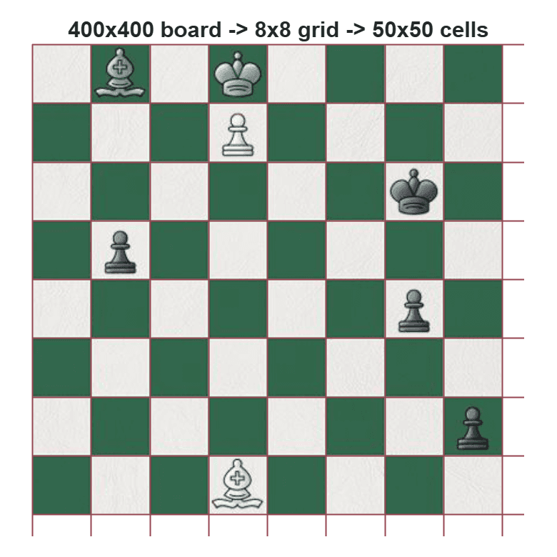
Everything runs on the koryakinp/chess-positions Kaggle dataset: 100,000 synthetically rendered 400×400 pixel chess boards with piece positions encoded as FEN strings in the filenames. From this single source, I generated two views. For the CNN: 6.4 million individual 50×50 cell crops labelled as one of 13 classes — empty square plus six piece types in two colours. For YOLO: bounding box annotations derived from the same grid. Same images, same split, same hardware. The only variable is the model.
Building the CNN from scratch
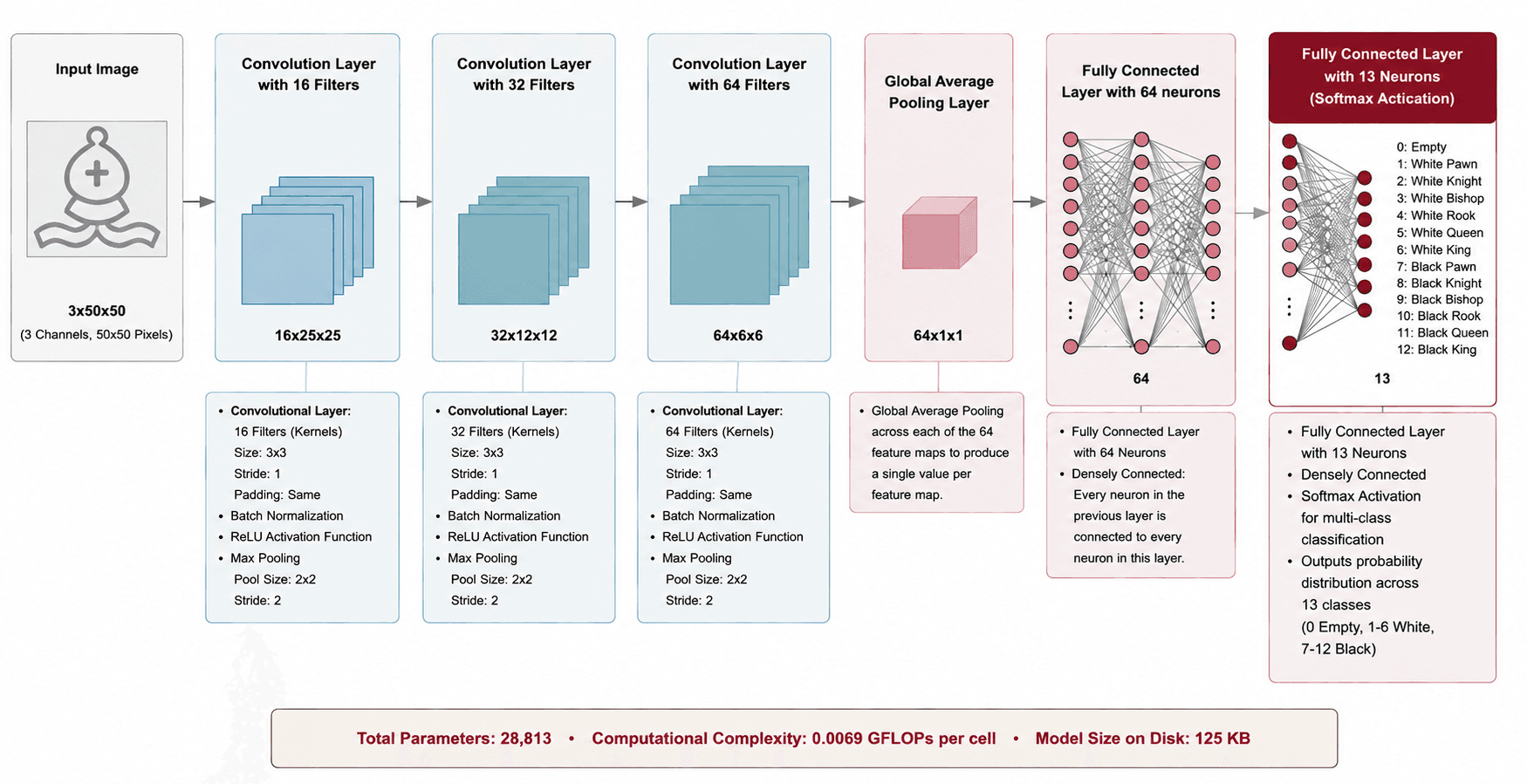
The custom CNN was designed through systematic hyperparameter search with Optuna, not intuition. Architecture depth, filter counts, learning rate, dropout — all optimised under a time budget with Weights & Biases tracking every trial. The final model is surprisingly compact: 34,513 parameters, 132 KB on disk. It does one thing — classify a 50×50 crop — and does it well. This is a classification task, not detection, so the CNN never has to find pieces — it just has to name them. That constraint is both its strength and its limitation.
YOLO enters the ring
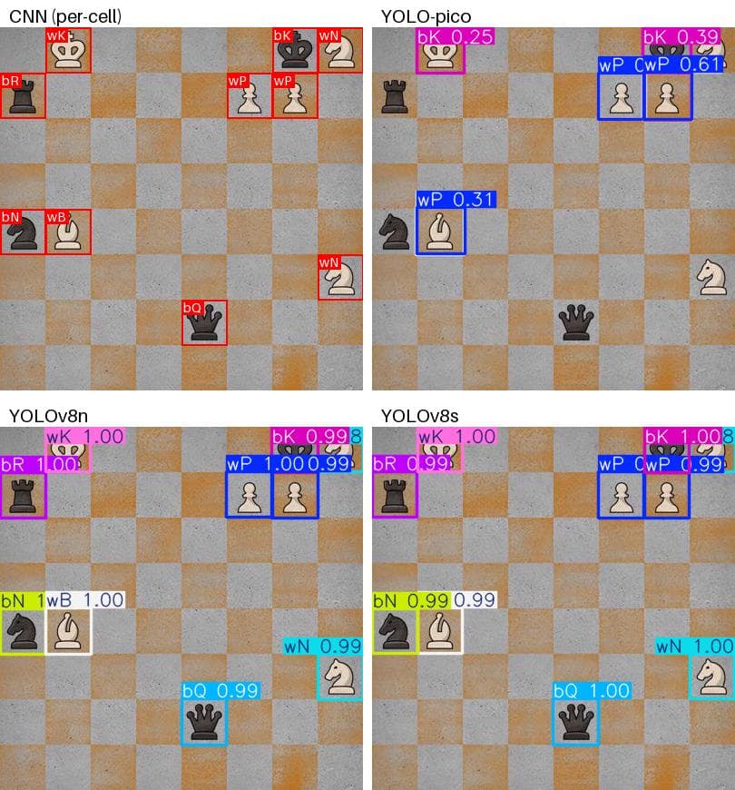
I trained three YOLOv8 variants — nano, pico, and small — on the same board images with bounding box annotations. YOLO has to do strictly more work than the CNN: find the pieces and identify them. That extra responsibility comes with overhead but also with a crucial advantage — YOLO processes the full board in one pass. No grid assumptions, no preprocessing pipeline to crop 64 cells per image. For real-world deployment where boards are photographed at angles and pieces are not on perfect grids, detection is more robust than classification.
What the numbers said
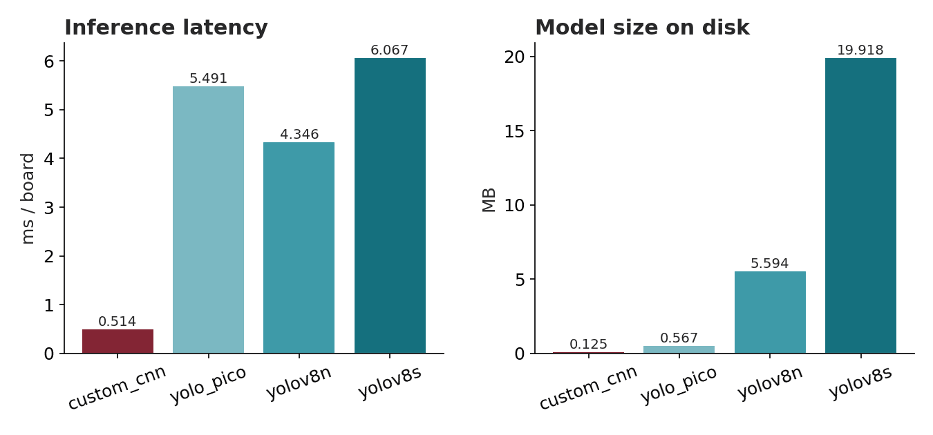
The full comparison — per-piece accuracy breakdowns, inference latency, parameter counts — is in the project report. But the short version surprised me: on this clean synthetic dataset, the CNN achieves 99.96% per-cell accuracy at 93× fewer parameters than YOLOv8n. It runs inference in 0.5 ms versus YOLO's 4–6 ms, and takes up just 0.125 MB versus YOLO-small's 20 MB. But YOLO, despite solving a harder problem, achieves strong results on full-board detection while being far more practical for deployment. The conclusion is not that one is better — it is that they answer different questions, and the right choice depends entirely on your deployment constraints.